INTRODUCTION TO A.I.

Bayes Rule and Bayesian Networks

March 8, 2007

8.1	Outline of Topics
	Probability
	Bayes Rule
	Example
	Bayesian Networks
	Bayesian Approach: Pros and Cons

8.2	Probability
	Probability	In case of uncertainty, probability is the "guess" that some proposition is true or false. This guess may sometimes be true and sometimes be false. If the guess is correct half of the time it is random and the probability is 0.5. ("Fifty-fifty" in daily speak.)
	Notation: P(e)	Given event e that we don't know whether happened, we use notation P(e) to refer to "the probability of event e happening" or "the probability of e or having happened". Without any further information, this is called the a priori or prior probability of e.
	∀e ∈ E: 0 <= P(e) <= 1	Probability is represented by a real number between 0 and 1.
	Prior probability: P(e)	For a set of atomic events/variables in a population of events E, a simple recording of their occurrence is their prior probability.
	Posterior probability: P(e\|D)	After we get the "evidence" (observed data) D, what is the probability of e?

8.3	Bayes rule
	Product rule	P(A ∧ B) = P(A)P(B\|A) P(A ∧ B) = P(B\|A)P(B)
	If we want to know	P(A\|B)
	We need to compute	P(B\|A), P(A), P(B)
	Bayes rule	P(A\|B) = P(B\|A)P(A) / P(B)
	Intuitively	P(B\|A): The higher the probability of A, the higher the probability of A given B P(A): The higher the probability of B given A, the higher the probability of A given B. P(B): The higher the probability of B in the absence of A, the less of a predictor of A is the presence of B. Hence it is the denominator.
	We need three terms	to compute the fourth
	Very often these three conditional terms can be computed before hand	For example, in medical diagnosis, computer vision, speech recognition

8.4

Example

Patient

has a particular form of hayfever or not

Patient has hayfever

Patient does not have hayfever

Laboratory test

Provides two outcomes, + and -

Lab test is not perfect

Outputs correct positive result in 98% of cases.
Outputs correct negative result in 97% of cases.
In other cases it returns the inverse result.

The percent of the population with this kind of hayfever

0.8%

The probabilities for this

The two hypotheses

Either the patient has hayfever or not

Case: We run the test on a patient

The result says: +

The less probable hypothesis, H1

P(+|hayfever)P(hayfever) = 0.98*0.008 = 0.0078

The more probable hypothesis, H2

P(+|¬hayfever)P(¬hayfever) = 0.03*0.992 = 0.0298

Alternative name for the most probable hypothesis

h_MAP (maximum a posteriori)

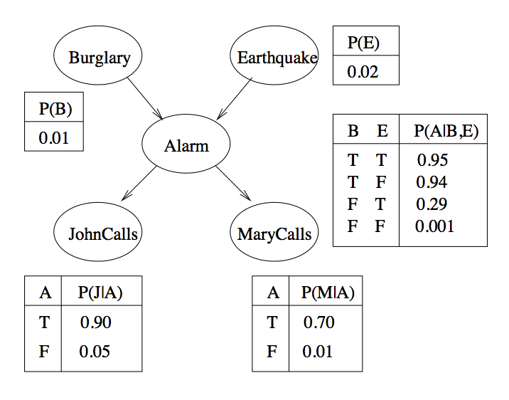
8.6

Bayesian Networks

Bayesian Belief Network

Directed acyclic graph, DAG - a directed graph with no cycles, e.g. A->B->C

Each state in the network has an associated conditional probability table

The table lists the conditional distribution for the variable given its immediate parents

Example conditional probability table for E→B→Q

More complex conditional probability table where B has two antecedents, E and W

B = Broadway show; E = Electricity; W = Weekend

The blue cell asserts

P(Broadway show = True | Electricty = True, Weekend = True) = 0.8

8.6	Bayesian Approach: Pros and Cons
	Pros	Can calculate explicit probabilities for hypotheses. Can be used for statistically-based learning. Can in some cases outperform other learning methods. Prior knowledge can be (incrementally) combined with newer knowledge to better approximate perfect knowledge. Can make probabilistic predictions.
	Cons	Require initial knowledge of many probabilities. Can become computationally intractable.